My first blobplot

1. Create a blobDB file from input files

1.1 Input file requirements

one assembly file, e.g. example/assembly.fna
one (or more) coverage file(s) e.g. example/mapping_1.bam
one (or more) hits file(s), e.g. example/blast.out

1.2 Creating a blobDB

# using the files provided in the test_files/ folder 
./blobtools create \
 -i example/assembly.fna \
 -b example/mapping_1.bam \
 -t example/blast.out \
 -o example/my_first_blobplot

2. Create a view of a blobDB file

2.1. Creating a view

Using blobtools view, information stored in a blobDB can be extracted.
Using the default settings, blobtools view will generate a tabular output for the taxonomic rank of "phylum".

./blobtools view \
 -i example/my_first_blobplot.blobDB.json \
 -o example/

2.2. Inspecting the output

The resulting file can be inspected using a one-liner (to indent the columns properly), e.g.:

grep '^##' example/my_first_blobplot.blobDB.table.txt ; \
 grep -v '^##' example/my_first_blobplot.blobDB.table.txt | \
 column -t -s $'\t'

## blobtools v1.0
## assembly	: example/assembly.fna
## coverage	: bam0 - example/mapping_1.bam
## taxonomy	: tax0 - example/blast.out
## nodesDB	: data/nodesDB.txt
## taxrule	: bestsum
##
# name     length  GC      N  bam0     phylum.t.6      phylum.s.7  phylum.c.8
contig_1   756     0.2606  0  90.406   Actinobacteria  200.0       0
contig_2   1060    0.2623  0  168.409  Actinobacteria  2300.0      0
contig_3   602     0.2342  0  43.761   Actinobacteria  10000.0     0
contig_4   951     0.3155  0  456.313  Actinobacteria  1000.0      0
contig_5   614     0.329   0  163.557  Nematoda        2000.0      0
contig_6   216     0.1944  0  25.88    Tardigrada      4000.0      2
contig_7   4060    0.2584  0  52.312   Nematoda        2000.0      0
contig_8   2346    0.2801  0  91.742   unresolved      2000.0      1
contig_9   1599    0.2439  0  74.757   Nematoda        200.0       0
contig_10  6273    0.3067  0  310.634  no-hit          0.0         None

The main header (##) contains version number, input files and parameters used while creating the blobDB file.
The table header (#) indicates the names of the columns (explained in the table below).
All following rows contain information about the sequences in the order they appear in the assembly file.

column header	description
name	name of the sequence
length	total length of the sequence, i.e. count(A, G, C, T, N)
GC	GC content percentage of the sequence, i.e. count(G, C)/count(A, G, C, T)
N	Number of N's in the sequence, i.e. count(N)
bam0	Coverage from bam0 (see main header for filename)
phylum.t.6	The assigned taxonomy of the sequence at the taxonomic rank of "phylum" under the tax-rule "best-sum"
phylum.s.7	The sum of scores for the taxonomy of the sequence at the taxonomic rank of "phylum" under the tax-rule "best-sum"
phylum.c.8	The c-index for the taxonomy of the sequence at the taxonomic rank of "phylum" under the tax-rule "best-sum"

If N > 1 coverage files are provided, N+1 coverage columns would show up in the table. One column per coverage files, and an additional column listing the sum of coverages across all files.
The last three columns list information about the taxonomy at the taxonomic rank of "phylum" under the tax-rule "best-sum".
If N > 1 taxonomic ranks are specified using the -r argument, additional columns will appear in the table.
If the --hits flag is used, the table will include the sum of scores by hits file for each taxID
The headers of the "taxonomy" columns are numbered (1-based) to ease filtering using command line applications such as GNU awk or UNIX/LINUX cut.

3. Create a blobplot

./blobtools plot \
 -i example/blobDB.json \
 -o example/

This generates three files:
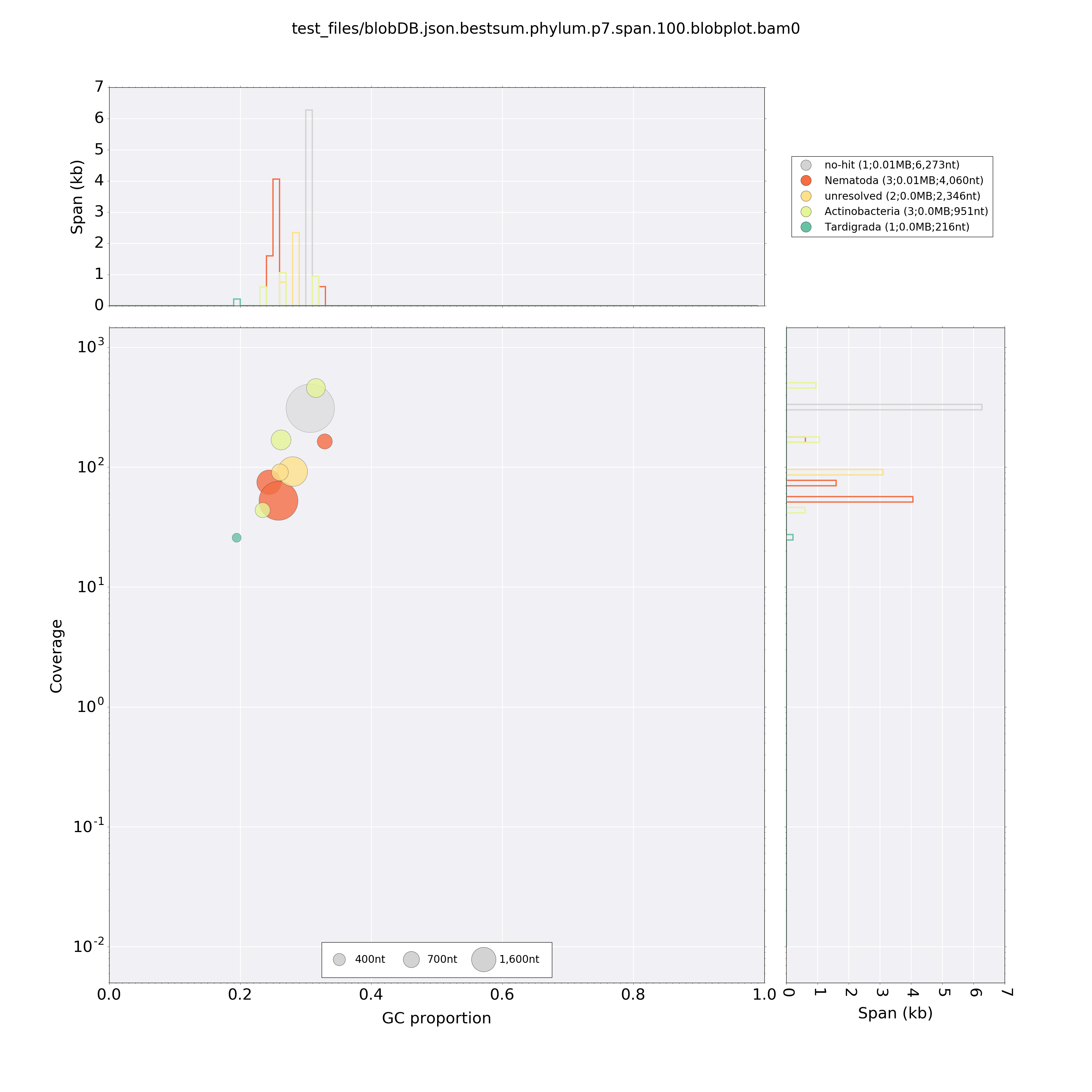
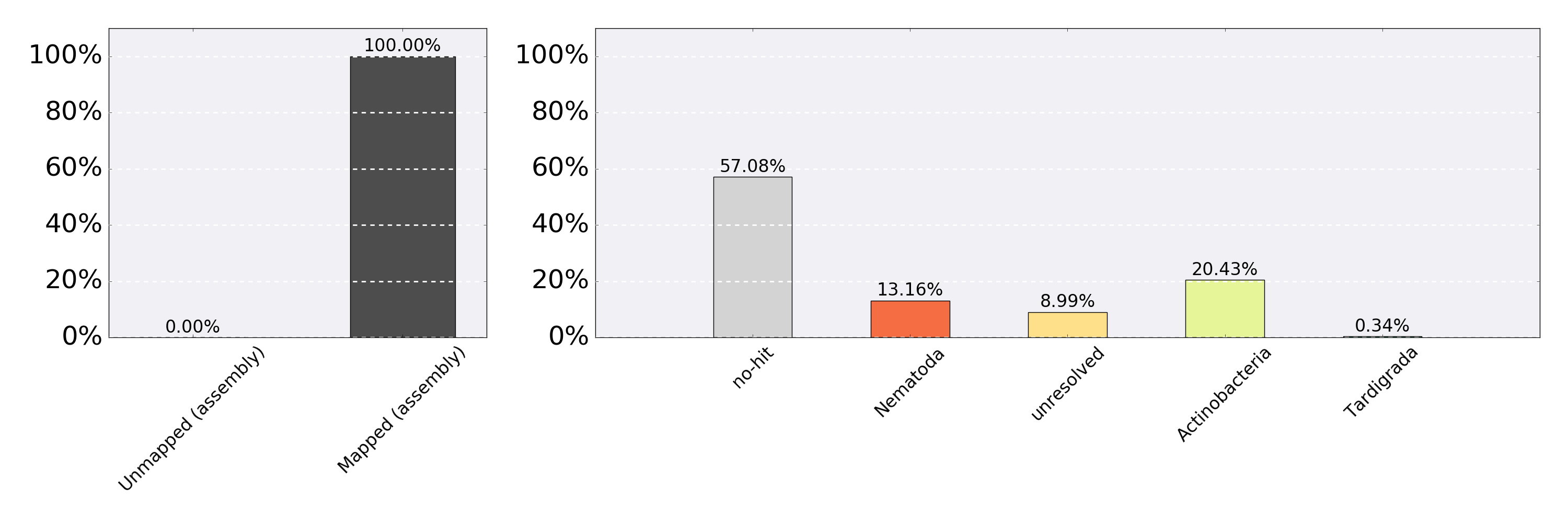
the blobplot blobDB.json.bestsum.phylum.p7.span.100.blobplot.bam0.png
the readcovplot blobDB.json.bestsum.phylum.p7.span.100.blobplot.read_cov.bam0.png
the stats file blobDB.json.bestsum.phylum.p7.span.100.blobplot.stats.txt

3000 — ReadCovPlot of example/blobDB.json